Three Body Simulation
One day I decided it would be nice to make a simulation of three planetary bodies. I wanted to write code that would run on Teensy microcontroler for the purpose of controlling eurorack synthesisir modules. The result would be 6 output voltages that represent the current X and Y coordinates of the three bodies.
This is how I went about writing the code to do this.
Coordinate system
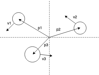
We will simulate the 3 bodies in 2 dimensions. The properties of each body, such as position, velocity and acceleration, will be represented by a 2D vector.
The origin of the system will be located at the centre of mass of the three bodies. This is becasue the centre of mass of any number of bodies always remains motionless.
The maths
Newton’s equations of motion
The 2 equations that we will need are, Newton’s second law:
\[F = ma\]and, Newton’s equation of universal gravitation:
\[F = \frac{Gm_{1}m_{2}}{r^2}\]The following equations use i and j subscripts to represent 2 of the three bodies.
- \(m_{i}\) is the mass of the first body.
- \(m_{j}\) is the mass of the second body.
- \(r_{ij}\) is the distance between the bodies.
- \(a_{i}\) is the acceleration of the first body.
Combining the equations of motion we can derive the following equation to calculate the force exerted on one body by another body:
\[F_{i} = m_{i}a_{i} = \frac{Gm_{i}m_{j}}{r_{ij}^2}\]To make acceleration a vector we can multiply the right hand side by a vector of length 1 representing the direction of body 2 in relation to body 1. To get a vector of length one we divide the vector by its length:
\[\frac{\vec{r_{ij}}}{r_{ij}}\]Combining with Newtons’s equations gives:
\[m_{i}\vec{a_{ij}} = \frac{Gm_{i}m_{j}}{r_{ij}^3}\vec{r_{ij}}\]We can then also divide each side by \(m_{i}\) to show the the mass of the first body does not contribute to it’s own acceleration:
\[\vec{a_{ij}} = \frac{Gm_{j}}{r_{ij}^3}\vec{r_{ij}}\]This gives the acceleration of one of the bodies caused by one of the other bodies. To get the accelaration of one body caused by the other two bodies we can simply add them together:
\[\vec{a_{1}} = \frac{Gm_{2}}{r_{12}^3}\vec{r_{12}} + \frac{Gm_{3}}{r_{13}^3}\vec{r_{13}}\]Euler method
From Newton’s equations, we can calculate an acceleration based on the positions of the bodies. We need to turn this into a velocity and a position and to do this we can use Euler’s method for solving differential equations. It uses a series of time steps to calculate the positions at certain points in time. It is the simplest way to approximate differential equations but also has the largest error, which is proportional to the size of the time step used.
It can be applied to the previous velocity and accelaration by multiplying by the time step size, \(\delta t\):
\[\vec{v}_{1} = \vec{v}_{0}+\vec{a} \delta t\] \[\vec{p}_{1} = \vec{p}_{0}+\vec{v} \delta t\]There are more accurate methods such as the Runge-Kutta method, but this is also more complicated and would require us to apply Newton’s equation multiple times for each sample. Since the code is designed to run on a microcontroller, we are trading speed for accuracy.
The code
We will use a vector class to store the various properties of a body and a Body class to store the current state. A Body has three variable properties; position, velocity, acceleration and one fixed scalar property; mass:
The class looks like this:
class Body {
    public:
        float mass = 1;
        Vector<2> position;
        Vector<2> velocity;
        Vector<2> acceleration;
};
The main simulation class called ThreeBody needs to have an array of 3 bodies and a time step variable:
class ThreeBody {
    ...
    private:
        Body bodies[3];
        float dt;
};
The bulk of the work is done in the calculateAcceleration function. This calculates the acceleration for a single body, the index being passed in as a parameter. It loops through the other bodies, and implements Newton’s equations to add each acceleration to the current bodies acceleration. The vector r is calculated as the difference between 2 bodies and the vector class provides a length function which uses Pythagoras’ equation to calculate the length.
void ThreeBody::calculateAcceleration(int i) {
    bodies[i].acceleration = Vector<2>(0, 0);
    for(int j = 0; j < BODIES; j++) {
        if(j != i) {
            Vector<2> r = bodies[j].position - bodies[i].position;
            float dist = r.length();
            bodies[i].acceleration += r * ((G * bodies[j].mass) / (dist*dist*dist));
        }
    }
}
Note the use of a Vector class with overriden operators means the calculation using vectors looks a lot easier to read than if we were dealing directly with x and y coordinates.
To put it all together, the main process function calls this for each body
void ThreeBody::process() {
    for(int i = 0; i < BODIES; i++) {
        calculateAcceleration(i);
    }
    ...
}
Then it applies Eulers method to each body by multiplying acceleration by the time step, then multiplying velocity by the time step to get the position.
for(int i = 0; i < BODIES; i++) {
    bodies[i].velocity += bodies[i].acceleration * dt;
    bodies[i].position += bodies[i].velocity * dt;
}
Initial conditions
The only thing that remains is setting of initial conditions. The initial conditions determine if the bodies fall into a stable orbit or not. In an unstable orbit the bodies will tend to fly apart eventually and never come back. It’s important to pick initial velocities with a net zero momentum, otherwise the system will drift away from the origin.
There are a few simple stable orbits we can create.
Lagrange points
Lagrange points are points in the standard orbit of 2 bodies (usually one massive like the sun and one smaller like the Earth), where a third body will form a stable orbit.
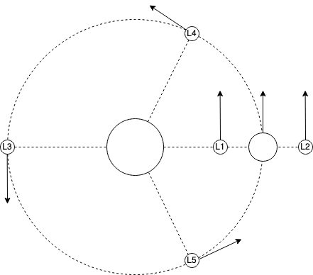
A simple lagrange L3 orbit can be produced by adding a large static body at the origin and two smaller bodies at either side with velocity in the opposite directions:
bodies[0].mass = 100;
bodies[0].position = Vector<2>(0, 0);
bodies[0].velocity = Vector<2>(0, 0);
bodies[1].mass = 1;
bodies[1].position = Vector<2>(0, 4);
bodies[1].velocity = Vector<2>(5, 0);
bodies[2].mass = 1;
bodies[2].position = Vector<2>(0, -4);
bodies[2].velocity = Vector<2>(-5, 0);
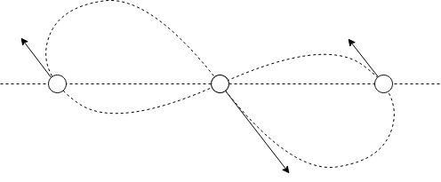
Figure 8 Orbit
Three equal bodies can be arranged to orbit in a figure of 8. The starting positions of the bodies should be on a line and equal distance from each other. The initial velocity vector of the centre body should be twice the magnitude and in the exact opposite direction of the outer bodies:
A handy function can be written to create a system like this.
void ThreeBody::initEqualInlineSystem(int mass, Vector<2> velocity) {
    bodies[0].mass = mass;
    bodies[0].position = Vector<2>(-1, 0) * mass;
    bodies[0].velocity = velocity;
    bodies[1].mass = mass;
    bodies[1].position = Vector<2>(1, 0) * mass;
    bodies[1].velocity = velocity;
    bodies[2].mass = mass;
    bodies[2].position = Vector<2>(0, 0) * mass;
    bodies[2].velocity = velocity * -2; // opposite and equal to other 2 velocities
}
Then we can experiment with different velocity directions. e.g. The following vector generates a stable figure of 8:
ThreeBody::initEqualInlineSystem(4, Vector<2>(0.347111, 0.532728));
And a more chaotic, but still stable, system is created with:
ThreeBody::initEqualInlineSystem(4, Vector<2>(0.210832, 0.51741));
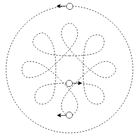
Broucke Orbit
A Broucke orbit looks like two bodies orbitings each other, which in turn are orbiting around a third body in a larger orbit.
Symmetrical stable version:
bodies[0].mass = 4;
bodies[0].position = Vector<2>(0.336130095, 0) * 4;
bodies[0].velocity = Vector<2>(0, 1.532431537);
bodies[1].mass = 4;
bodies[1].position = Vector<2>(0.7699893804, 0) * 4;
bodies[1].velocity = Vector<2>(0, -0.6287350978);
bodies[2].mass = 4;
bodies[2].position = Vector<2>(-1.1061194753, 0) * 4;
bodies[2].velocity = Vector<2>(0, -0.9036964391);
Asymmetrical stable version:
bodies[0].mass = 4;
bodies[0].position = Vector<2>(-2.855484,-0.099324);
bodies[0].velocity = Vector<2>(-0.14822,-0.47005);
bodies[1].mass = 4;
bodies[1].position = Vector<2>(-1.785072,0.406224);
bodies[1].velocity = Vector<2>(-1.47620,1.02377);
bodies[2].mass = 4;
bodies[2].position = Vector<2>(4.640556,-0.306904);
bodies[2].velocity = Vector<2>(-0.20557,1.39997);
More complex stable orbits can be created, but these tend to destabilise over a short time due to errors introduced by the approximate nature of the Euler method used.
Possible Improvements
Because of the low accuracy of the integration method used, it may not be possible to simulate some of the more complex orbits with them becoming unstable quickly. One possible way of improving the accuracy is to use an adaptive time step. Since the bodies tend to travel faster when closer together we could try reducing the time step when the bodies are closer together.
Another thing we could do if we are interested in keeping an orbit stable is to reset the simulation to the exact initial conditions after we know that one complete orbit should have been made. This would prevent the second ‘lap’ of the orbit from being slightly different to the first and building up error over time.