Musical Tuning
In order to understand why we generally use 12 equally spaced notes in musical scales, I put together some visualisations which show the notes/intervals against dissonance/consonance curves.
The Python code used to generate the plots can be found here
It’s generally known that the most consonant intervals in music are where the difference in frequencies of 2 notes played together can be expressed as simple ratios. e.g. an octave is a ratio of 2/1, which means the root note with frequency of say 440Hz is played at the same time as a note with double the frequency, 880Hz. A perfect fifth is the ratio of 3/2 which puts the note frequency at 660Hz.
Instead of using frequency ratios it’s easier to visualize this on a linear scale where the root note is a 0 and the octave is at 1. Then 2 octaves would be 2.
Ratios can be converted using the base 2 logarithm, e.g the perfect fifth:
\[log_2(3/2) = 0.585\]To convert from octaves back to ratio you can raise 2 to the power of the value:
\[2^{0.585} = 1.5 = 3/2\]To get from an octave value to a frequency, the following equation can be used:
\[f = a2^{v}\]where $a$ is the root frequency and $v$ is the octave value.
Tuning is often expressed in cents, where each semitone in the 12 tone scale is divided by 100. Octaves can easily be converted to cents by multiplying by 1200:
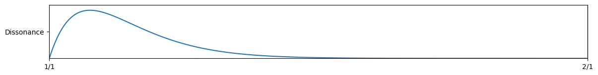
\[0.585 \times 1200 = 702\]Dissonance Curve
The curve below shows the dissonance of 2 sine waves played at increasing frequency intervals. The curve is based on experimental results by Plomp and Levelt in the paper Tonal Consonance and Critical Bandwidth. It shows that consonance is greatest when the 2 sine waves are at the same frequency. As the frequency interval increases it become more dissonant, after a level of maximum dissonance it then drops off again to become gradually more consonant.
from lib.tuning import Tuning
from lib.tuningplot import TuningPlot, TuningPolarPlot
%matplotlib inline

plot = TuningPlot('h', 14)
plot.plotDissonance([1], 1)
plot.plotRatios([(1, 1), (2, 1)])
plot.plot()
Harmonic Series
Unlike sine waves, most real word musical sounds comprise of frequencies in the harmonic series. That is they have frequencies that are an integer multiple of a fundamental frequency.
A dissonance curve can be calculated by adding up all the dissonances between pairs of partials in a particular sound. See Relating Tuning and Timbre by William Sethares.
For instance the following curve is plotted from a sound with the first 6 harmonics:
plot = TuningPlot('h', 14)
plot.plotDissonance([1, 2, 3, 4, 5, 6])
plot.plotRatios([(1, 1), (2, 1), (3, 2), (4, 3), (5, 3), (5, 4), (6, 5)])
plot.plot()
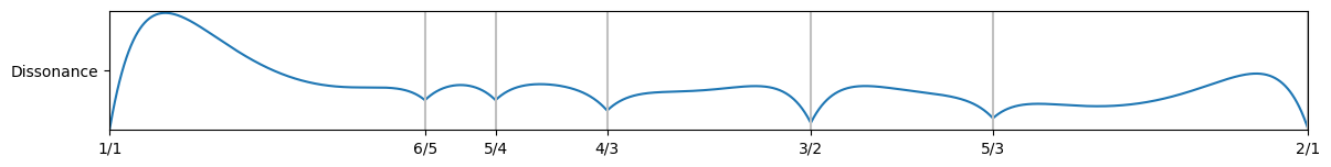
You can see from this that the most consonant intervals are representated by simple ratios, which are also marked on the graph.
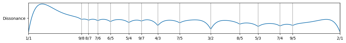
This is how the curve changes when more partials are added:
plot = TuningPlot('h', 14)
plot.plotDissonance([1, 2, 3, 4, 5, 6, 7, 8, 9], 5.5)
plot.plotRatios([(1, 1), (2, 1), (3, 2), (4, 3), (5, 3), (5, 4), (6, 5), (7, 4), (7, 5), (7, 6), (8,5), (8,7), (9, 5), (9, 7), (9, 8)])
plot.plot()
The most common tuning in western music is the 12 tone equal temperament or 12 Equally Divided Octave (12edo) tuning, which divides the octave into 12 equal intervals. Being equally divided adds the convenience that music can be easily transposed on an instrument while sounding the same without having to retune to change keys.
The following graph shows these 12 intervals against the dissonance curve:
tuning_12edo = Tuning.createEqualDivisionTuning("12edo", 12, 1, ['0 C','1 C#','2 D','3 D#','4 E','5 F','6 F#','7 G','8 G#','9 A','10 A#','11 B'])

plot = TuningPlot('h', 14)
plot.plotRatios([(1, 1), (2, 1), (3, 2), (4, 3), (5, 3), (5, 4), (6, 5), (7, 4), (7, 5), (8,5), (9, 8), (9, 5)])
plot.plotDissonance([1, 2, 3, 4, 5, 6, 7, 8, 9], 5.5)
plot.plotTuning(tuning_12edo)
plot.plot()
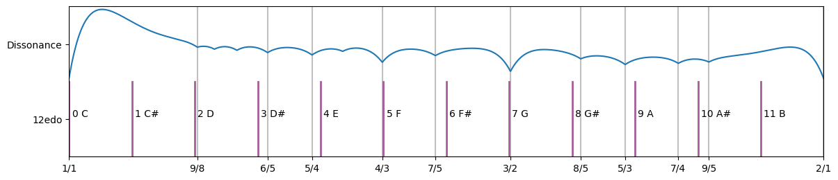
The most consonant intervals, the Perfect Fifth (3/2) and the Perfect Fourth (4/3) match notes on this scale nearly perfectly, which makes it quite useful. Other consonant intervals are slightly off, but the human ear can tolerate small differences in pitch without noticing too much.
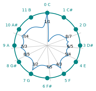
Plotting in intervals around a circle reveals an almost symmetrical pattern of simple ratios. Most of the intervals have inverse versions e.g. 1/2 - 3/2 = 4/3, or an octave minus a fifth is equal to a fourth.
plot = TuningPolarPlot(4, 4, 2, 1)
plot.plotRatios([(1, 1), (3, 2), (4, 3), (5, 3), (5, 4), (6, 5), (7, 4), (7, 5), (8,5), (8,7)])
plot.plotTuning(tuning_12edo)
plot.plotDissonance([1, 2, 3, 4, 5, 6, 7, 8], 5.5)
plot.plot()
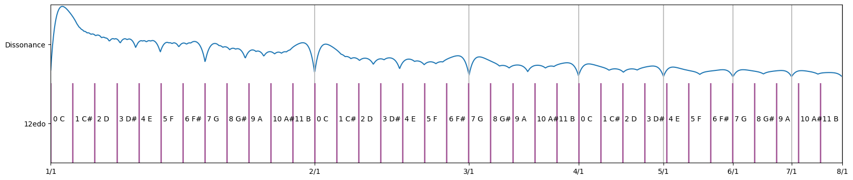
If the dissonance curve is extended beyond the octave then consonant dips can be seen which match the harmonic series.
- The graph shows 3 octaves starting at 1/1. The second ocatve starts at 2/1, the third at 4/1 to 8/1
- The differences between adjacent harmonics follows a pattern:
- (2/1) / (1/1) = 2/1 (Octave)
- (3/1) / (2/1) = 3/2 (Fifth)
- (4/1) / (3/1) = 4/3 (Fourth)
- (5/1) / (4/1) = 5/4 (Major Third)
- (6/1) / (5/1) = 6/5 (Minor Third)
plot = TuningPlot('h', 20, 3)
plot.plotDissonance([1, 2, 3, 4, 5, 6, 7, 8, 9, 10, 11, 12, 13, 14, 15], 8)
plot.plotRatios([(1, 1), (2, 1), (3, 1), (4, 1), (5, 1), (6, 1), (7, 1), (8, 1)])
plot.plotTuning(tuning_12edo, 3)
plot.plot()
Alternative Tunings
There are other equal divisions of the octave that can be used to match other intervals closer than 12edo.
The graph below shows a scale with 19 equal divisions.
tuning_19edo = Tuning.createEqualDivisionTuning("19edo", 19, 1)

plot = TuningPlot('h', 14)
plot.plotRatios([(1, 1), (2, 1), (3, 2), (4, 3), (5, 3), (5, 4), (6, 5), (7, 4), (7, 5), (7, 6), (8,5), (9, 8), (9, 7), (9, 5)])
plot.plotDissonance([1, 2, 3, 4, 5, 6, 7, 8, 9], 5.5)
plot.plotTuning(tuning_12edo)
plot.plotTuning(tuning_19edo)
plot.plot()
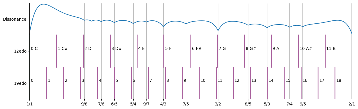
This scale deviates slightly from 3/2 and 4/3 but matches nearly perfect with 6/5, 5/3 and more closely to 5/4, 8/5 and also has a note near 9/7 which has no close equavalent in 12edo.
If we used 19edo to make music, standard concepts from 12edo like the heptatonic scales and major and minor chords, would need to replaced with new concepts. The easiest thing to do would be to translate the notes to the nearest notes in 19edo, but it should also be possible to experiment with new types of chord from these more consonant intervals. The difficulty in inventing a whole new musical system leaves alternative tunings largely unexplored.
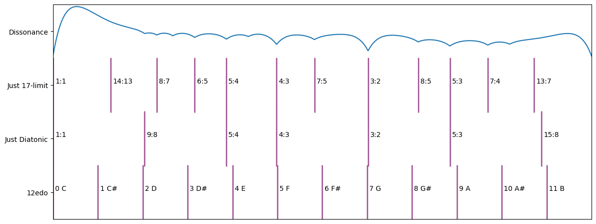
Just Intonation
Just intonation throws away the requirement for equaly spaced notes infavour of more consonant intervals. Tuning physical instruments to a just intonations limits the ability to change key and transpose music, but electronically generated music doesn’t have to have this limitation as it has the potential to be transposed out of scale.
There are many ways of creating just scales, some prefer simpler ratios over trying to match 12edo closely, others prefer larger ratios in favour of getting closer to 12edo.
A couple of examples are shown below, but there are many more examples on the Wikipedia page - Just intonation.
tuning_justdiatonic = Tuning("Just Diatonic", [])
tuning_justdiatonic.addIntervalRatio(1, "1:1")
tuning_justdiatonic.addIntervalRatio(9/8, "9:8")
tuning_justdiatonic.addIntervalRatio(5/4, "5:4")
tuning_justdiatonic.addIntervalRatio(4/3, "4:3")
tuning_justdiatonic.addIntervalRatio(3/2, "3:2")
tuning_justdiatonic.addIntervalRatio(5/3, "5:3")
tuning_justdiatonic.addIntervalRatio(15/8, "15:8")

tuning_just17limit = Tuning("Just 17-limit", [])
tuning_just17limit.addIntervalRatio(1, "1:1")
tuning_just17limit.addIntervalRatio(8/7, "8:7")
tuning_just17limit.addIntervalRatio(5/4, "5:4")
tuning_just17limit.addIntervalRatio(4/3, "4:3")
tuning_just17limit.addIntervalRatio(3/2, "3:2")
tuning_just17limit.addIntervalRatio(5/3, "5:3")
tuning_just17limit.addIntervalRatio(13/7, "13:7")
tuning_just17limit.addIntervalRatio(14/13, "14:13")
tuning_just17limit.addIntervalRatio(6/5, "6:5")
tuning_just17limit.addIntervalRatio(7/5, "7:5")
tuning_just17limit.addIntervalRatio(8/5, "8:5")
tuning_just17limit.addIntervalRatio(7/4, "7:4")

plot = TuningPlot('h', 14)
plot.plotDissonance([1, 2, 3, 4, 5, 6, 7, 8, 9], 5.5)
plot.plotTuning(tuning_just17limit)
plot.plotTuning(tuning_justdiatonic)
plot.plotTuning(tuning_12edo)
plot.plot()
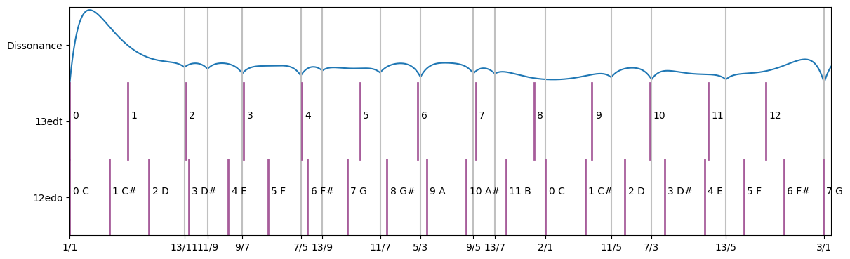
Odd Harmonics
For a sound with only odd harmonics, such as a square waves and triangle waves, the dissonance curve looks quite different.
plot = TuningPlot('h', 14, 1.6)
plot.plotDissonance([1, 3, 5, 7, 9, 11, 13], 3.3)
plot.plotRatios([(1, 1), (2, 1), (3, 1), (5, 3), (7, 5), (7, 3), (9,5), (9,7), (11,7), (11,9), (11,5), (13,7), (13,9), (13,11), (13,5)])
plot.plot()
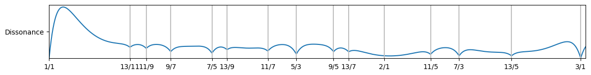
Here there is a consonant dip at 3/1 interval which is an octave (2/1) plus a fifth (3/2):
\[log_2(2/1) + log_2(3/2) = log_2(3/1)\] \[2/1 \times 3/2 = 3/1\]The interval 3/1 can be called a tritave (Also a perfect twelfth, but this name is based on step sizes in 12 edo).
Note also, there is no peak at the fifth like the other graphs.
These intervals fit better with a 13 note equally divided tritave. This is the basis of the Bohlen-Pierce scale.
tuning_13edt = Tuning.createEqualDivisionTuning("13edt", 13, 1.585)

plot = TuningPlot('h', 14, 1.6)
plot.plotDissonance([1, 3, 5, 7, 9, 11, 13], 3.3)
plot.plotRatios([(1, 1), (2, 1), (3, 1), (5, 3), (7, 5), (7, 3), (9,5), (9,7), (11,7), (11,9), (11,5), (13,7), (13,9), (13,11), (13,5)])
plot.plotTuning(tuning_13edt)
plot.plotTuning(tuning_12edo, 2)
plot.plot()