Musical Sequence Generation in Eurorack Using a Variational Autoencoder

This is a document describing how I trained a variational autoencoder on musical sequences and perform inference in a Eurorack module.

All training code is in the xen_machinelearning repository.

Code and hardware design used for inference on a Teensy microcontroller based Eurorack module can be found in the xen_quantizer repository.

Variation Autoencoder Architecture

A variational autoencoder (VAE) to a type of neural network. A VAE learns to encode complex data into a lower-dimensional space (latent space) and then decode it back to the original data space. New data can then be generated by sampling from the latent space.

The input of the encoder is a fixed length sequence of boolean values which represet a fixed length sequence of musical notes. e.g. If notes are represented by points on a grid with pitch vertically and time horizontally, the input to the VAE is a flattened version of this.

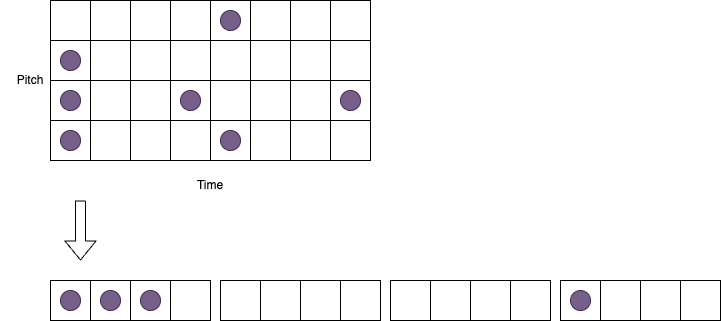
The VAE has an input for each note per tick of the clock, so the total number of inputs is notes x ticks.

Training is done by presenting the same input data as output data. The bottleneck in the VAE causes it to find a low dimensional representation of the input. In this case 3 numbers are all that are needed to represent a particular piece of input data.

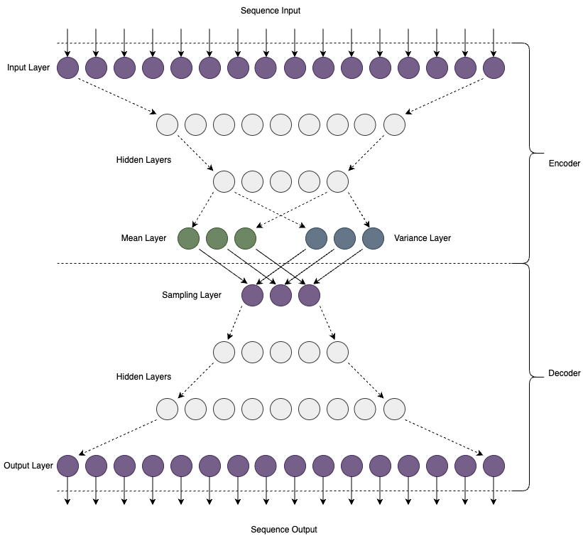
Once the VAE is trained the decoder part of the network is converted to tflite which is a format that we can use on hardware. The latent variables can be set directly from a potentiomer or control voltage input to generate a new sequence.

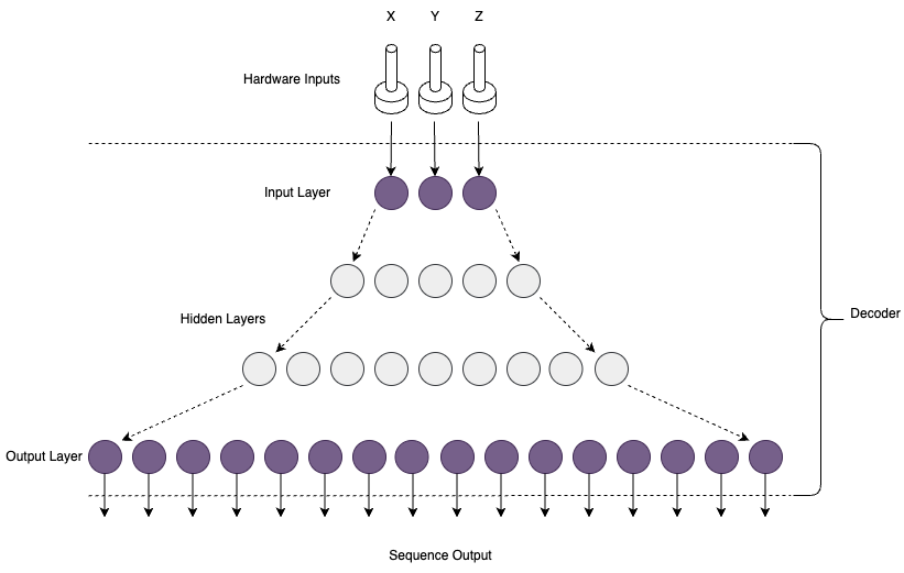
The output sequence is then converted back into a time based sequence by splitting it up and fed to the outputs based on an external clock pulse.

Percussion mapping

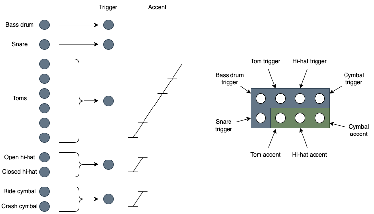
Percussion sequences are handled slightly differently to sequences of musical notes. Instead of using pitch we just map each instrument to a different row in the sequence. Because the number of trigger outputs is limited in hardware we map midi instrument numbers to smaller subset of intruments.

We can group intruments based on a standard drum kit into 12 outputs. During inference these 12 outputs are further grouped into a set of 5 trigger outputs, and 3 accent outputs. This process is illustrated in the diagram below:

Percussion instruments can of course be grouped in many different ways. Various different percussion maps can be used and are defined in the file PercussionMap.py

Training

Training is done on a batch of midi files. The xen_machinelearning repository contains handy functions for filtering and converting midi files to the required sequence format.

Since the sequence length has to be a fixed size for the VAE we need to decide the length of each sequence to train it on. The midi files are cut up into sections of a fixed length, with a measure of music being a convenient length. We also want to filter the data to specific time signature to ensure the bar lengths we are training on are constant. e.g. We can filter all measures with a 4/4 time signature and encode them as 16 step sequences, each step representing 1/16th note. Parts of music with name ‘Percussion’ can also be exluded.

paths = ["/path/to/midi/files"]
instrumentFilter = NameFilter(exclude="Percussion")
trainer = SequenceVAETrainer(modelPath="../models", modelName="note_model_16")
trainer.loadSongDataset(paths, timesig='4/4', ticksPerQuarter=4, quartersPerMeasure=4, measuresPerSequence=1, instrumentFilter=instrumentFilter)

In the above code we are loading a directory of midi files and filtering it to 4/4 time signature, and encoding to sequences of 1 measure length, with 4 quarter notes per measure and 4 steps or ticks per quarter note, making a total sequence length of 16 (4 * 4 * 1).

To train a model on percussion sequences instead we include all parts with the name ‘Percussion’ and pass a percussion map object to tell the model how to group the percussion instruments.

paths = ["/path/to/midi/files"]
instrumentFilter = NameFilter(include="Percussion")
trainer = SequenceVAETrainer(modelPath="../models", modelName="perc-model_16")
trainer.loadSongDataset(paths, timesig='4/4', ticksPerQuarter=4, quartersPerMeasure=4, measuresPerSequence=1, instrumentFilter=instrumentFilter, percussionMap=ExtendedPercussionMap)

If any of the sequences left after filtering contain notes which don’t adhere the sequence constraints, then those measures will also be discarded. e.g. triplets cannot be represented by a sequence length of 16, if those were to be included then ticksPerQuarter would need to be 12, making the sequence length 12 * 4 * 1 = 48

Once the data is loaded the VAE model can be created with:

trainer.createModel(latentDim = 3, hiddenLayers = 2)

The latentDim is the number of dimensions in latent space which will correspond to the 3 inputs during inference. The hiddenLayers is the number of layers we want to add between the input and latent layers. The size of the hidden layers will be automatically calculated to produce a linear size decrease from input to latent layers.

latentScale can also be set, this sets the range of numbers that latent space can be. e.g. setting a value of 3 will ensure the latent values are somehwere beteen -3 and +3. 3 is the default value.

All that remains is to train the model and save it:

trainer.train(batchSize = 32, epochs = 500, learningRate = 0.005)
trainer.saveModel(quantize = None)

The values of these parameters can be experimented with. POssible parameters are:

• batchSize: The number of sequences in each batch of training
• epochs: The total numer of training steps to go through
• learningRate: The rate at which the network learns
• patience: If the loss is not reduced after this nmber of epochs then the learning rate is automatically lowered. Defaults to 100
• factor: The amount that the learning rate is lowered by. Defaults to 0.5
• minLearningRate: Traning will stop if the learning rate goes below this number. Defaults to 0.000001

During training the loss will be displayed. The aim is to get the loss as low as possible. If the loss is not going down much then it may be because there is too much of a range of data to learn everything with the size of the current model. To remedy this the amount of training data can be reduced, or the number of hidden layers or latent space size can be increased. However, larger models will lead to longer inference times and increasing the number of latent dimension will require changes to the number of inputs during inference (since this will be implemented in hardware it will be difficult to increase this without hardware redesign).

After training the model will be saved as a complete VAE (***_vae.h5) as well as a tflite file containing just the decoder to be used by microcontroller inference.

Verification

There are a few functions that can be used to check if the model is well trained.

trainer.calcRecall()

This calculates how well the trained model is able reproduce the training data. A recall of 50% represents no training at all as even a compeltely random output will be correct 50% of the time for each element. Values of above 50% mean that training has worked correctly.

trainer.plotLatentSpace()

This will plot a 2 dimensional graph of each dimension of latent space against each of the other dimensions. It should produce an output a bit like this:

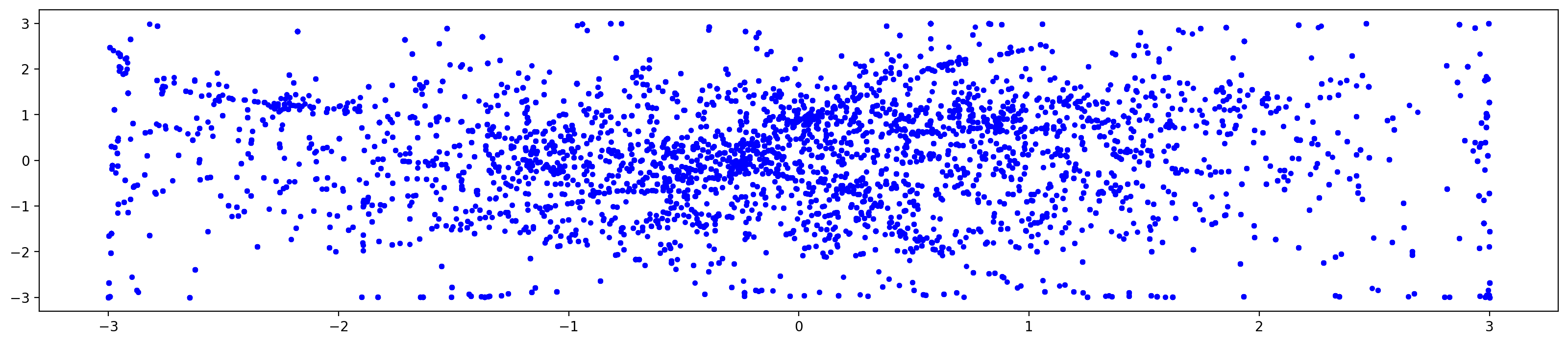
Ideally the latent points are evenly spread over the entire latent space. You can see that the latentScale setting has constrained the upper and lower bounds to -3 and +3.

Clusters of points show the points in space where there are more similar sequences in the training data.

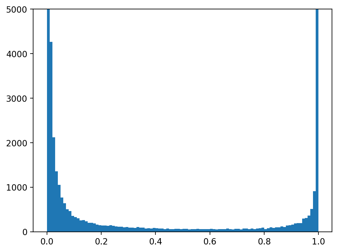
trainer.plotOutputValueDistribution()

This plots the range of output values. The value of each output will be a number between 0 and 1 to indicate the probablity that that pitch is triggered. Most values should be around 0 and 1 with a dip in the middle.

trainer.plotInputOutputSequence(1, threshold = 0.5)

This funnction can be used to plot a specific training example at the input and output. The first number is the index of the sequecne in the training data, you can change it to any number to pull out different examples. The resulting 2 plots should look similar to indicate that the input is simlar to the output.

Model Metadata

The tflite format has a very limited set of metadata that can be saved in the model, so a sequence of bytes is embedded in the decription field of the tflite file. This metadata is needed during inference and has the following format:

content	length (bytes)	description
string “seqdec”	6
number of pitches	1	Number of possible notes in each time step
sequence length	1	Total length of the sequence
latent scale	1	The range of values that each latent dimension can be. e.g. a value of 3 means the latent value can be netween -3 and +3.

Some extra metadata is required for percussion models:

content	length (bytes)	description
string “perdec”	6
number of instruments	1	Number of possible notes in each time step
sequence length	1	Total length of the sequence
latent scale	1	The range of values that each latent dimension can be. e.g. a value of 3 means the latent value can be netween -3 and +3.
number of groups	1	Number of percussion grouops represented in the output
group sizes	number of groups	The number of instruments in each percussion group

Hardware inference

The xen_quantizer repository contains hardware design and code for inference using the trained tflite model.

The model file can be read from an SD card. There are seperate controllers for pitches sequences and drum sequences. Model fiels for each are read from the directories /models/note/ and /models/perc respectively.